What you will understand
- The band depends on the volatility assumptions supplied.
- A pointwise percentile line is not one simulated business path.
- A simulated reserve-breach share is not a calibrated probability of failure.
What simulation adds to a fixed scenario
A deterministic scenario answers what follows from one set of assumptions. A Monte Carlo simulation repeats a calculation with varied inputs to explore a conditional range of results. It can expose how a range changes when assumptions about variation change, but it does not remove the need to justify those assumptions.
The important word is conditional. A model with arbitrary volatility, missing cash movements or unrealistic relationships can still draw a convincing band. Before reading the percentiles, ask what varied, how it varied and what remained fixed.
The 500-path example and its explicit assumptions
The starting scenario has EUR 10,000 cash, monthly revenue of EUR 20,000, monthly costs of EUR 16,000, six months, no growth and no collection delay. The reserve is EUR 5,000. Without variation, the scenario ends at EUR 34,000.
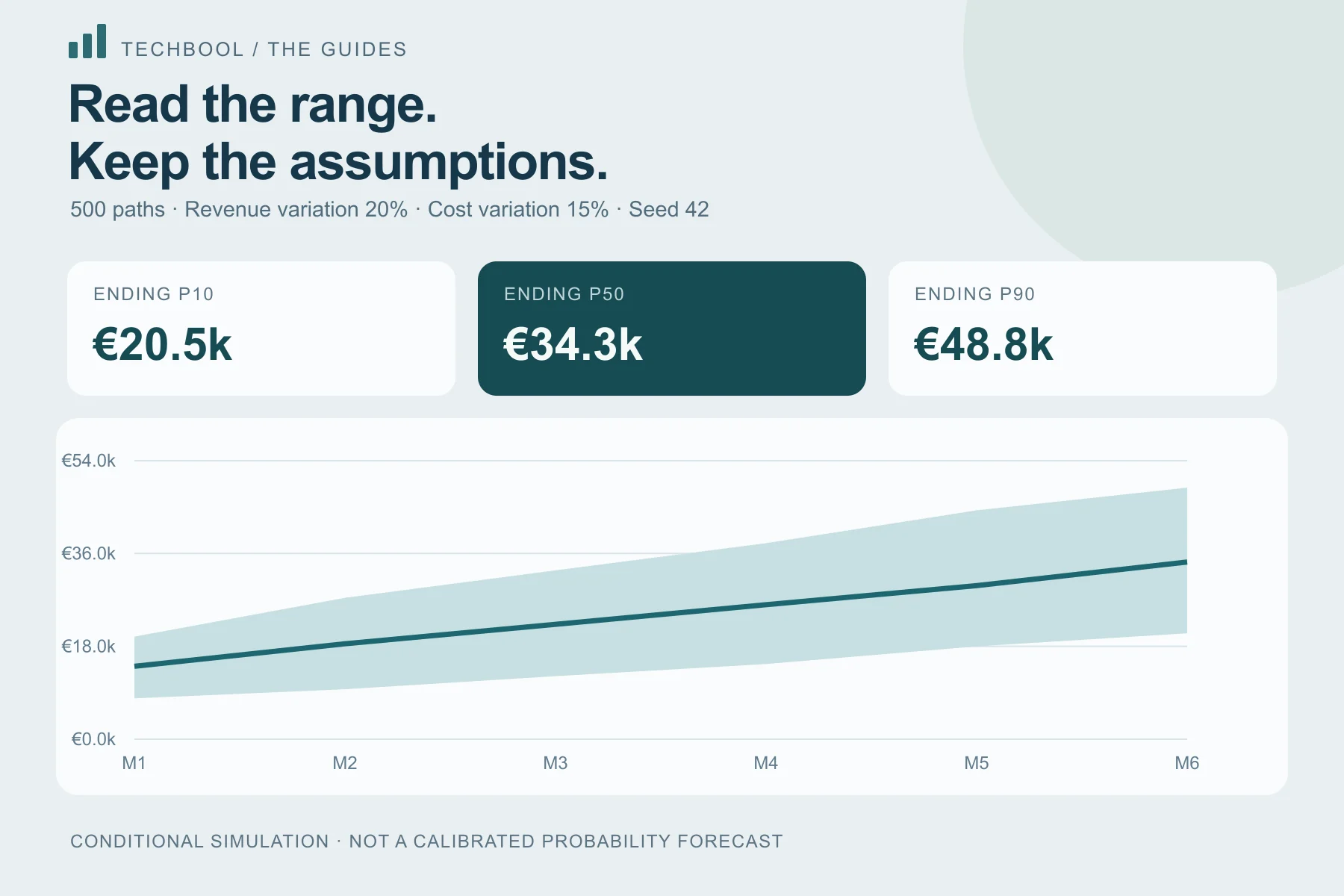
For this illustration, revenue volatility is 20% and cost volatility is 15%, with random seed 42. These are user-chosen standard-deviation assumptions, not estimates inferred from the CSV. Techbool applies independent normal monthly multipliers to nominal revenue and cost, clips negative multipliers at zero and runs 500 paths.
The calculation preserves the saved growth, shocks, opening cash and collection delay. It does not estimate correlations, seasonality, customer concentration or structural changes. Independence is a modelling assumption, not an observation about real revenue and costs.
| Setting | Value |
|---|---|
| Paths | 500 |
| Revenue standard deviation | 20% |
| Cost standard deviation | 15% |
| Seed | 42 |
| Projection | 6 months |
| Reserve | EUR 5,000 |
Read P10, P50 and P90 as positions in simulated outcomes
For each month, Techbool sorts the 500 closing balances. P50 is the middle of that empirical distribution. P10 and P90 mark lower and upper positions using linear interpolation. The band describes outputs of this simulation under its assumptions.
In the final month of this reproducible illustration, P10 is EUR 20,532.16, P50 is EUR 34,348.44 and P90 is EUR 48,767.15. They do not establish an 80% real-world confidence interval. The model has not demonstrated that its chosen input distribution matches the future business.
The median need not equal the deterministic baseline exactly. Finite sampling, rounding and clipping can shift it. A saved seed makes the calculation repeatable; it does not make its assumptions more accurate.
| Measure | Value |
|---|---|
| Ending P10 | EUR 20,532.16 |
| Ending P50 | EUR 34,348.44 |
| Ending P90 | EUR 48,767.15 |
| Paths with a month-end reserve breach | 25 of 500 (5%) |
A percentile line is not one coherent path
The balance at the tenth percentile in month one may belong to a different path from the tenth percentile in month six. Joining pointwise percentiles produces a useful summary, but the joined line is not necessarily a path any simulation actually followed.
Do not take the P10 value in every month and describe the sequence as one specific downside business case. If you need an explainable operational case, build a deterministic scenario with a coherent set of revenue, cost and timing assumptions, then inspect its complete timeline.
Interpret the reserve-breach percentage narrowly
Here, 5% of 500 paths have at least one projected month-end below the EUR 5,000 reserve. That is 25 generated paths, not a measured 5% probability the company will fail. A reserve breach is not the same event as insolvency, and these input assumptions have not been calibrated as a probability model of the company.
The monthly table answers a different question: what share of paths is below the floor in that particular month? A path can appear in more than one monthly count. Adding monthly percentages therefore does not produce the share that breached at least once.
Even if no generated paths breached a reserve, that would not prove the event impossible. A finite sample can miss rare outcomes, and the model may exclude the mechanism creating the risk. Use the result to ask better questions, not to make an unconditional safety claim.
Challenge assumptions before comparing two bands
Change one modelling choice at a time. First examine whether the volatility inputs are supported by relevant history or a clearly described stress question. Then consider whether independent revenue and cost variation makes sense. If a sales drop is usually accompanied by a margin change, independent noise can miss that relationship.
Keep the horizon, currency, reserve and starting scenario consistent. A wider band can come from a longer horizon or larger variation; it does not automatically mean a different business is inherently riskier. Label changed assumptions beside the chart.
More generated paths do not repair an omitted mechanism. If a single large customer determines receipts, or one known payment dominates the cash position, an explicit scenario for that event may be more informative than adding random noise around an average.
- Record the source and meaning of chosen volatility.
- Consider whether known events matter more than random variation.
- Keep deterministic cases alongside percentile summaries.
- State omitted taxes, financing, capital spending and correlations.
- Avoid presenting conditional sample shares as guaranteed probabilities.
Save and inspect the calculation in Techbool
Risk simulation is a Pro feature. Open a saved scenario in Decision lab, choose the two volatility inputs and seed, and save the analysis. The result includes its assumptions, calculation version, monthly percentile table and conditional reserve-breach shares. JSON preserves the complete record; CSV and printing support review.
For specific revenue and cost combinations, a sensitivity matrix is often easier to explain than a random simulation. Choose the simpler analysis when it answers the decision. Additional computation is useful only when its assumptions and output remain understandable.
Keep the inputs.
Understand the outcome.
Start with a Free workspace. Inspect the calculation and compare a second scenario before choosing a paid analysis tool.